In my first spreadsheet tutorial, I described how I wanted to take this information from iTunes:

and calculate the average song length. If you read that tutorial, you know that the average length of each item in my iTunes library (including podcasts) turned out to be 246.9675647 seconds. In this tutorial, we’ll find out how to turn that into information that is useful to a regular human being.

Since we’ve already covered the basics of entering formulas and functions, I’ll skip over most of that. Instead, we’ll look at a couple of more advanced functions.

Converting Seconds to Minutes

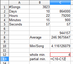
The easiest thing to do is to convert seconds into minutes. In B10, I typed “Minutes/Song” and in B11 I entered an equal sign to indicate that we will be doing some calculations. I then clicked in cell C8, typed the division sign (/), and entered 60:

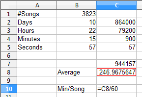
Hitting the enter key gives us:

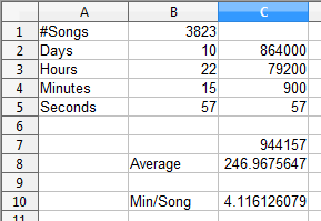
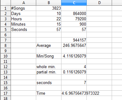
so our average time is approximately 4.11 minutes per song.

Displaying Seconds as Seconds

A song length of 4.11 minutes is far more useful to the average human than a song length of 246.97 seconds, but time is usually displayed in a combination of minutes and seconds, not one or the other. In order to do this, we need to follow a three-step process:

1. Separate the whole minutes (4) from the partial minutes (0.116126079).
2. Convert the partial minutes into seconds.
3. Recombine minutes and seconds.

This is actually easier than it looks.

Separating Whole Minutes from Partial Minutes

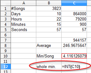
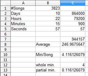
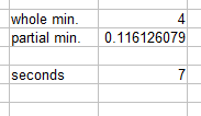
Spreadsheets have a function, `INT()`, which will round any number down to the nearest whole number. In our case, it will give us the whole minutes. In C12, I entered `=INT(C10)`:

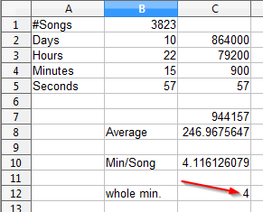
Hitting the enter key gives us our integer, which in this case is 4:

To get those partial minutes, we’ll just subtract that whole minute from our original figure. The formula I used is `=C12-C10`:

Hitting the enter key gives us the value we were looking for:

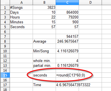
Multiplying that value by 60

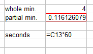
gives our seconds as seconds:

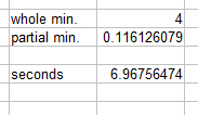
That’s still a long number. We need to round it off. We could use the `=INT()` function again, but let’s learn how to format cells a bit.

First, we’ll right click on the cell in question. That brings up this contextual menu*:

We’ll select “Format Cells…” which brings up this dialogue box:

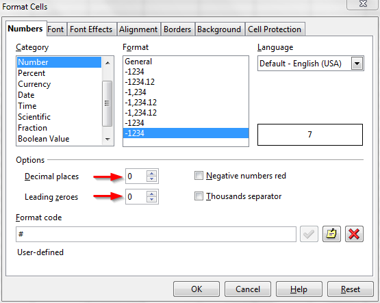
Under “Category” we’ll select “Number” because these cells contains numbers. Under “Options” we’ll set both “Decimal places” and “Leading zeroes” to 0. I added arrows in the above screen cap to highlight this.

Clicking “OK” closes the dialogue box and gives us the result we were looking for:

Combine Minutes and Seconds

Now we just need to put those together so that they appear like this: `4:07`. We can do this using the `=CONCATENATE()` function.

`=CONCATENATE()` is a handy function for formatting your output, taking whatever input you hand to it and stringing it together like beads on a string.

Again, the format is the same: equal sign, function, arguments in parentheses separated by semicolons:

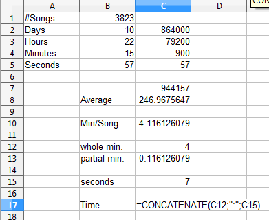
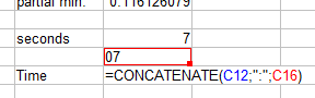
In this case, the formula I used was `=CONCATENATE(C12;”:”;C15)`. I had to include the semicolon between quotation marks.

Hitting the enter key gives us this:

Now that is exactly not what we wanted. If you recall, we formatted the seconds to display a number with no places after the decimal. However, we only formatted C15 that way. That format won’t affect other cells that the data from C15 is copied over to.

What we need is a way to specify the precision of the data in C15 that will carry over to other cells. We already have a function, `=INT()` that will strip off the decimal portion, but that won’t work for us. Our value is very close to 7, and `=INT(C15)` would give us a value of 6. We need a function that will round values to whatever level of precision we want.

As it turns out, the function that does that is `=ROUND()`. We can apply that to C7, and that information will carry over to C17:

Hitting the enter key gives us what we’re looking for:

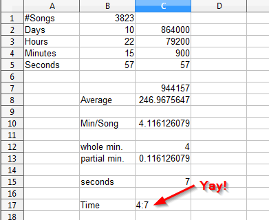
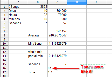
Except that’s not what we want, either. In time notation, the second number (in this case, the seconds) should always be written with two digits. That really should look be 4:07.

We could use the `=CONCATENATE()` function to add a zero in front of there, but if the seconds were two digits already, we would end up with three digits for the seconds, instead of two. What we need is a function that will add a leading zero only if the value is less than ten.

As it turns out, the function that will do that for us is the `=IF()` function. It has three parts:

1. A test that is either true or false.
2. What to do if the test is true.
3. What to do if the test if false.

In our case, these parts look like this:

1. The seconds are less than ten.
2. Add an extra zero when displaying the seconds.
3. Display the seconds the way they are.

Again, the arguments are separated by semicolons. To make it easy to keep track of things, let’s put this in a separate cell:

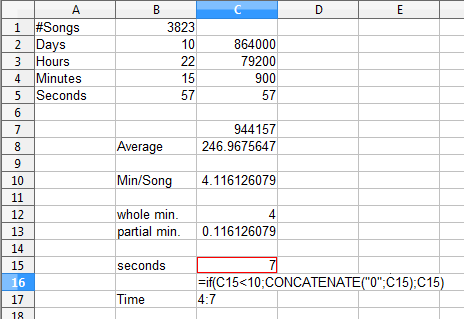
Again, hitting the enter key gives us what we were looking for:

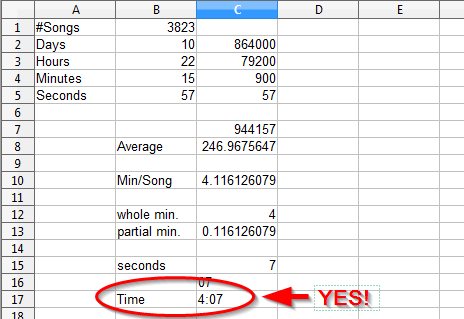
So now we can link to C16 in C17:

 

Which gives us what we were looking for in the first place:

Nested Functions

If you look closely at C16, you can see that we’ve included the `=CONCATENATE()` function inside the `=IF()` function. This is called a nested function.

I suppose there is some logical limit built into OpenOffice or even Windows as to how deeply we can nest functions, but it is unlikely that we will ever need to nest them 6 or 7 deep. We could, for example, nest the formula from C16 into the formula in C17:

`=CONCATENATE(C12;”:”;IF(C15<10;CONCATENATE(“0”;C15);C15))`

Note that when we nest a function, we omit the equal sign. That only occurs once in each cell, at the very beginning of the formula.

In reality, it can become difficult to keep track of all those nested functions. It’s usually easier to put all of those functions in their own row or column and then hide them. We can even put them in a separate worksheet. There are advantages and disadvantages to both of those methods, but we’ll cover those in a later tutorial.